[논문 리뷰] Understanding Diffusion Models: A Unified Perspective (3)

Understanding Diffusion Models: A Unified Perspective는 3가지 포스트로 나누어져 있습니다. 이전 포스팅을 참고해주세요.

 

Paper: https://arxiv.org/abs/2208.11970

Understanding Diffusion Models: A Unified Perspective

 

1. ELBO, VAE, HVAE

https://donghyun99.tistory.com/14

[논문 리뷰] Understanding Diffusion Models: A Unified Perspective (1)

 

2. Variational Diffusion Models

https://donghyun99.tistory.com/16

[논문 리뷰] Understanding Diffusion Models: A Unified Perspective (2)

 

---

Score-based Generative Models

지난번 포스트에서는 VDM이 neural network인 $s_\theta(x_t, t)$를 통해 score function인 $\nabla \log{p(x_t)}$를 심플하게 예측할 수 있다는 것을 보여주었습니다. 다만 이것은 Tweedie's Formula를 통해 예측한 값을 대입해준 것일 뿐 score function에 대한 정확한 insight가 없습니다. 

 

따라서 이번에는 Score-based Generative Model을 통해 score function이 어떤 식으로 계산되는지를 알아보겠습니다. 결론적으로 보면 VDM이 유도하는 수식과 동일하지만 해석의 방향성으 조금 다릅니다.

 

Energy-based Models

Score-based generative Models을 알기 위해서는 Energy-based Models에 대한 이해가 필요합니다. Energy-based Models은 Yann LeCun이 자세하게 설명한 ppt가 있습니다.

http://www.cs.toronto.edu/~vnair/ciar/lecun1.pdf

 

내용을 요약해보겠습니다.

 

위의 그림은 이미지에 대한 Classification을 하는 Task입니다. 즉 우리는 $X$에 대한 알맞는 $Y$를 찾아내는 것을 목표로 합니다. Energy는 $X$와 $Y$를 어떠한 공간에 대한 좌표 축으로 봤을 때, 각 샘플들이 매핑되는 하나의 Scalar 값을 의미합니다.

이때 Energy Function은 데이터 분포가 큰 곳은 Energy가 더 적고, 반대로 분포가 적은 곳에 대해서는 Energy가 더 커지도록 에너지를 생성하는 것을 학습합니다. Supervised 기반 학습에서는, 어떻게 보면 Loss 함수의 값과 비슷합니다. 데이터 분포가 몰려있는 쪽의 Loss가 더 낮으니까요. (저는 그렇게 이해했습니다.)

 

Energy-Based GAN(EBGAN)은 Discriminator를 Energy Function으로 보고 높은 분포의 입력은 낮은 값을, 낮은 분포의 입력은 높은 값을 출력하도록 모델을 구성했습니다. 단순히 real/fake를 1,0으로 분류하는 기존의 모델들과는 차별점이 있는 방식이였죠. Discriminator를 Auto Encoder로 만들어 입력 이미지를 복원시키고, 복원된 이미지와 입력 이미지 사이의 MSE Loss를 Energy로 사용하였습니다.

 

Energy-Based GAN

 

이제 다시 Score-based Model로 돌아와서 생각해봅시다. Score-based Model은 이 Energy에 대한 개념을 Loss가 아니라 확률 분포(Probability Distributions)에 대한 개념으로 생각해야 합니다.

 

$$p_{\theta}(x)=\frac{1}{Z_{\theta}}e^{-f_{\theta}(x)} \tag{152}$$

 

$f_\theta(x)$는 neural network로 모델링된 energy based function이며 $Z_{\theta}$는 $\int{p_\theta(x)}dx=1$이여야 하기 때문에 이를 위하기 위한 normalization 상수 입니다. Energy가 낮을 수록 $p(x)$의 값은 높아지기 때문에 위에서 생각한 energy의 개념과 같습니다.

 

다만 Maximum Likelihood 방법을 사용하기 위해서는 $Z_\theta=\int{e^{-f_\theta(x)}}dx$인 상수를 쉽게 계산할 수 있어야 합니다. 그렇지만 딱히 방법이 없기 때문에 우리는 $Z_\theta$를 무시하고 근사할 수 있는 방법을 생각해야 합니다.

 

Score function을 근사한 신경망 $s_\theta(x)$에 대한 표현으로 나타내 봅시다.

 

$$\begin{align} \nabla_{\boldsymbol{x}} \log p_{\boldsymbol{\theta}}(\boldsymbol{x}) & =\nabla_{\boldsymbol{x}} \log \left(\frac{1}{Z_{\boldsymbol{\theta}}} e^{-f_{\boldsymbol{\theta}}(\boldsymbol{x})}\right) \tag{153} \\ & =\nabla_{\boldsymbol{x}} \log \frac{1}{Z_{\boldsymbol{\theta}}}+\nabla_{\boldsymbol{x}} \log e^{-f_{\boldsymbol{\theta}}(\boldsymbol{x})} \tag{154} \\ & =-\nabla_{\boldsymbol{x}} f_{\boldsymbol{\theta}}(\boldsymbol{x}) \tag{155} \\ & \approx \boldsymbol{s}_{\boldsymbol{\theta}}(\boldsymbol{x}) \tag{156} \end{align}$$

 

위와같이 Normalization 상수를 포함하지 않고 표현이 가능합니다. GT score function에 대한 fisher divergence는 다음과 같습니다.

 

$$\mathbb{E}_{p(x)} \bigg[ ||s_\theta(x)-\nabla \log{p(x)}||^2_2 \bigg] \tag{157}$$

 

 

Fisher Divergence

 

Fisher Divergence는 확률 분포간 차이를 측정하는 방법 중 하나입니다. KL Divergence와 비슷한 개념이지만 KL Divergence는 비대칭적이고 Fisher Divergence는 대칭적인 성질을 가지고 있습니다. Fisher Divergence의 수식은 다음과 같습니다.

 

$$F(p, q) = \frac{1}{2}\bigg(\text{Tr}(Cov(q)^{-1} Cov(p))+(\mu_q-\mu_p)^T Cov(q)^{-1}(\mu_q-\mu_p)-k+\ln{\frac{\det(Cov(q))}{\det(Cov(p))}}\bigg)$$

 

$Cov$는 공분산 행렬, $\text{Tr}$은 행렬의 대각 요소의 합입니다. $\det$는 determinant로 행렬식입니다. 즉 p와 q의 평균과 공분산을 이용해 두 분포사이의 거리를 측정합니다. Eq 157은 아마 이를 간단하게 표현한 것 같습니다.

 

 

---

 

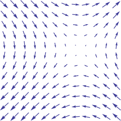
우리는 모든 $x$에 대한 likelihood를 높임으로써 dataspace에서 어떤 방향으로 이동해야되는지를 학습합니다. score function은 dataspace에서 mode를 가리키는 vector field를 정의하는 역할을합니다. 말이 좀 어려운데 mode는 최빈값을 나타내고 (GAN의 단점이라 할 수 있는 mode collapse의 mode입니다.) vector field는 아래 그림을 보면 바로 이해가 될 것 같습니다.

https://en.wikipedia.org/wiki/Vector_field

Vector field - Wikipedia

 

Vector field는 흐름의 크기와 방향을 나타낸 지도라고 생각할 수 있습니다. true data distribution의 score function을 학습하여 mode에 도달할 때까지 반복적으로 표본을 생성합니다.

 

위의 그림은 score function을 통해 정의된 vector field를 따라 mode를 찾아가는 모습을 시각화 한 것입니다.

표본을 추출하는 프로세스는 Langevin dynamics를 사용합니다.

 

Langevin Dynamics (랑주벵 동역학)

 

Brownian motion(브라운 운동)은 입자들이 불규칙하게 운동하는 현상입니다. 여기서 Langevin Dynamics는 브라운 운동을 수학적으로 모델링한 미분 방정식(differential equation)입니다.

Brownian motion

 

https://ko.wikipedia.org/wiki/%EB%B8%8C%EB%9D%BC%EC%9A%B4_%EC%9A%B4%EB%8F%99

브라운 운동 - 위키백과, 우리 모두의 백과사전

https://en.wikipedia.org/wiki/Langevin_equation

Langevin equation - Wikipedia

브라운 운동에 대한 Langevin Dynamics는 다음과 같이 정리할 수 있습니다.

 

$$F=m\ddot{x}=-\lambda \dot{x}+\eta$$

 

$m$은 입자의 속도이고 $\lambda$는 damping coefficient(감쇠 계수)이며 $\eta \sim \mathcal{N}(0,2\sigma^2)$는 Gaussian noise입니다. (F는 Force 즉 힘입니다.)

 

질량이 m인 입자에 대한 Force F

 

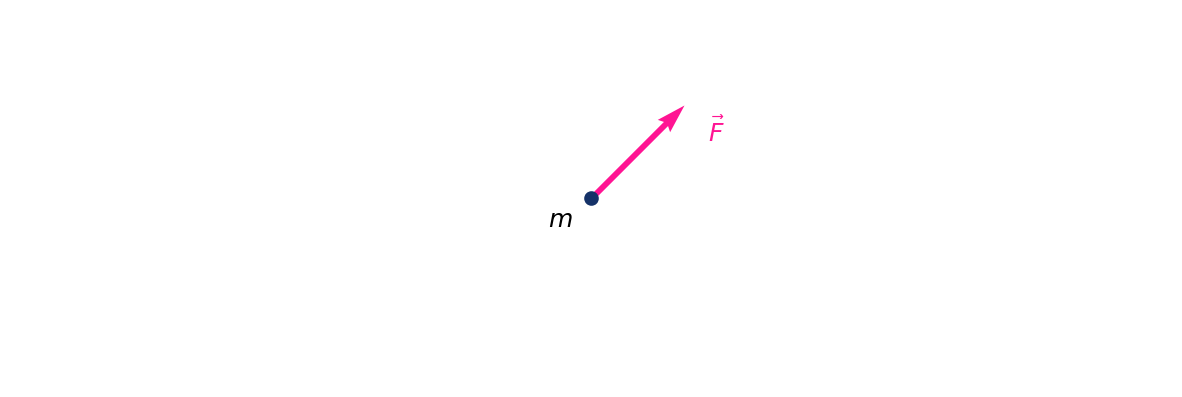
이때 물리에서 입자의 Force($F$)는 Potential energy $V(x)$의 미분으로 나타낼 수 있습니다. 수식을 정리하면 아래와 같이 나타낼 수 있습니다.

 

$$\begin{aligned} m \ddot{x} &= F = \frac{\partial V(x)}{\partial x}=\nabla V(x) \\ \nabla V(x) &=-\lambda\dot{x} + \eta \\ \lambda \dot{x} &=-\nabla V(x) + \eta \end{aligned}$$

 

여기에 Stochastic Differenctial Equation (SDE)를 넣으면 다음과 같이 나타낼 수 있습니다.

 

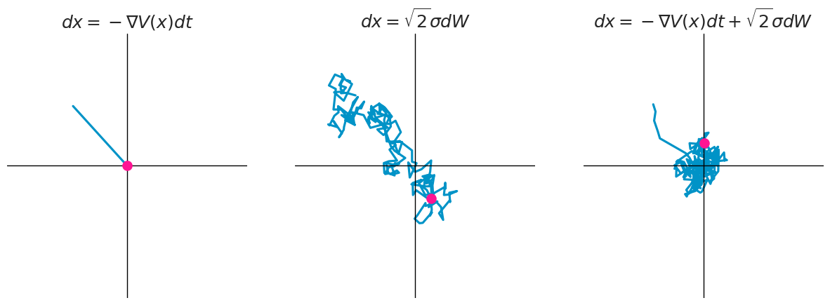
$$dx=\underbrace{-\nabla V(x)dt}_{\text{drift term}}+\underbrace{\sqrt{2}\sigma dW}_{\text{diffusion term}}$$

 

여기서 $-\nabla V(x)$는 drift term, $\sigma$는 Volatility(변동성), 그리고 $dW$는 표준 Weiner process의 시간 t에따른 도함수(미분)입니다. 음.. 자세히는 모르겠지만, 확실한건 $\sigma dw$는 이 식의 불확실성을 의미하고 무작위의 diffusion에 대한 force를 의미한다는 것입니다. 다음 그림을 보시면 직관적으로 이해할 수 있습니다.

 

potential energy, random force, 그리고 두개를 합쳤을 때에 대한 Langevin dynamics의 확산과정.

 

SDE는 따로 확률미분방정식에 대한 공부가 없다면 이해하기 힘들 수 있습니다. 아래 블로그에 잘 설명되어 있으니 혹시 더 정확한 수학적 설명을 원하시면 참고해 주세요.

https://freshrimpsushi.github.io/categories/%ED%99%95%EB%A5%A0%EB%AF%B8%EB%B6%84%EB%B0%A9%EC%A0%95%EC%8B%9D/

확률미분방정식

 

---

 

Steady State of Langevin Dynamics

 

Langevin dynamics을 통해 분포로부터 표본을 추출하기 위해서는 Langevin dynamics가 생성하는 분포($q(x, t)$)를 특정할 수 있어야 합니다. 이를 위해 시간에 따른 확률 밀도함수의 미분 방정식인 Fokker-Planck equation을 이용해봅시다.

먼저 Standard Wiener process $W$를 통해 구현된 Itô process(이토 확률 과정)의 가장 기본적인 SDE는 다음과 같습니다:

 

$$dx=\mu(x,t)dt + \sigma(x,t)dW$$

 

앞서 나온 SDE에서는 여기에 $-\nabla V(x)$와 $\sqrt{2}\sigma$를 대입한 것입니다. 여기서도 마찬가지로 $\mu(x,t)$는 drift term, $\sigma(x,t)$는 Volatility입니다.

 

여기서 우리는 $D(x,t)=\sigma(x,t)^2/2$를 diffusuion coefficient(확산 계수)라고 정의하겠습니다. 이때 위의 SDE에 대한 Fokker-Plank equation은 다음과 같이 정의됩니다:

 

$$\frac{\partial}{\partial t}p(x,t)=-\frac{\partial}{\partial x}[\mu(x,t)p(x,t)]+\frac{\partial^2}{\partial x^2}[D(x,t)p(x,t)]$$

 

https://en.wikipedia.org/wiki/Fokker%E2%80%93Planck_equation

Fokker–Planck equation - Wikipedia

 

우리는 $p(x,t)$를 알 수 없기 때문에 $q(x,t)$를 통해 수식을 나타내야 합니다. $p(x,t)=q(x,t)$를 대입하고 마찬가지로 이전 SDE에서 대입한 $\mu(x,t)=\nabla V(x)$와 $\sigma(x,t)=\sqrt{2}\sigma$를 통해 Langevin Dynamics의 식으로 고쳐봅시다.

 

$$\frac{\partial}{\partial t}q(x,t)=\frac{\partial}{\partial x}[\nabla V(x)q(x,t)]+\frac{\partial^2}{\partial x^2}[\sigma^2q(x,t)]$$

 

식이 유도되었습니다!! 위 식에서는 x와 t라는 변수가 있네요. 이 Fokker-Plank equation을 x와 t에 대해 시뮬레이션한 그래프를 그려보면 아래 그림과 같이 나타나게됩니다.

 

시간에 따른 q(x,t)의 분포. 두 개의 Gaussian Distribution은 시간이 지나면서 분포가 일정하게 수렴하게 됨.

 

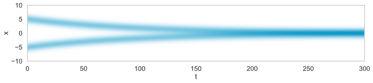
그림을 보면, t가 커짐에 따라 x가 0으로 수렴하게 됩니다. 이때 그래프의 기울기는 0이 될테니 $\frac{\partial}{\partial t}q(x,t)=0$이되겠죠? 이 때 $\underset{t\to\infty}{\lim}{\ q(x,t)}=q_{\infty}(x)$라 합시다. 그리고 아래와 같이 가정하고 식을 정리해봅시다.

 

$$\lim_{t \to \infty}q(x,t)=q_\infty(x) \\ \frac{\partial}{\partial t}q_\infty(x)=\frac{\partial}{\partial x}\bigg[\nabla V(x)q_\infty(x)+\frac{\partial}{\partial x}[\sigma^2q_\infty(x)]\bigg]=\frac{\partial}{\partial x}J=0$$

 

여기서 J는 Probability current(확률 흐름)이라고 하며, 임의의 공간 x에 대한 확률밀도의 흐름의 정도를 나타내는 값입니다. 그냥 $\bigg[\nabla V(x)q_\infty(x)+\frac{\partial}{\partial x}[\sigma^2q_\infty(x)]\bigg]$를 나타내는 정도로만 이해합시다. 어쨌든 우리는 위의 그래프에서 t가 무한대일 때, $q_\infty(x)$의 미분만 0에 수렴하는 것이 아니라 값 도 0에 수렴하는 것을 알 수 있습니다. 즉 모든 $x$에 대하여 $J(x)=0$입니다. 그렇다면 다음과 같이 식을 유도할 수 있습니다.

 

$$\begin{aligned} J(x)=\bigg[\nabla V(x)q_\infty(x)+\frac{\partial}{\partial x}[\sigma^2q_\infty(x)]\bigg]&=0 \\ \frac{\partial}{\partial x}[\sigma^2q_\infty(x)]&=-\nabla V(x)q_\infty(x) \\ \frac{\partial}{\partial x}q_\infty(x)&=-\frac{\nabla V(x)}{\sigma^2}q_\infty(x) \end{aligned}$$

 

$q_\infty(x)$를 미분했는데 $q_\infty(x)$가 있는 식이 나오네요. 그렇다면 $q_\infty(x)$는 $e^{f(x)}$꼴의 함수라고 추측할 수 있습니다.

$\frac{\partial}{\partial x}e^{f(x)}= \nabla[f(x)] e^{f(x)}$이기 때문입니다. 그렇다면 $q_\infty(x)$에 대한 완전한 함수를 정의하는 것은 힘들더라도 비례식은 세울 수 있습니다 $\nabla V(x)$는 $V(x)$의 미분이고, $\sigma$를 상수 취급했을 때 다음과 같은 비례식을 유도할 수 있습니다:

 

$$q_\infty(x) \propto \text{exp}\bigg( -\frac{V(x)}{\sigma^2} \bigg)$$

 

위의 비례식은 Boltzmann distribution(혹은 Gibbs distribution)의 비례식과 같습니다.

https://en.wikipedia.org/wiki/Boltzmann_distribution

Boltzmann distribution - Wikipedia

 

그렇다면 비례식에서 normalization constant인 $Z$를 통해 비례식이 아닌 방정식으로 나타낼 수 있습니다. Energy-based models의 form처럼 바꾸자면, 우리가 실제로 추정하는 $p(x)$에 대하여, $p(x)= \frac{exp[-V(x)]}{Z}$ 입니다. ($V(x)=E(x)$즉 Energy Function 이기 때문에 이같은 형태로 정의가 가능합니다.) 다음과 같이 정리할 수 있습니다.

 

$$\begin{aligned} p(x) = \frac{exp[-V(x)]}{Z} \\ \log{p(x)} = \log{\frac{exp[-V(x)]}{Z}} \\ \log{p(x)} = \log{\frac{1}{Z}} + \log{exp[-V(x)]} \\ \log{p(x)} - \log{\frac{1}{Z}} = \log{exp[-V(x)]} \\ V(x) = -\log{p(x)} + \log{\frac{1}{Z}} \\ \nabla V(x)=-\nabla\log{p(x)} \end{aligned}$$

 

$Z$는 상수이기 때문에 미분 시 0입니다. 앞서 제시한 SDE의 drift term에 대입하여봅시다.

 

$$dx = \nabla\log{p(x)dt}+\sqrt{2}\sigma\nabla W$$

 

---

 

Sampling Using Langevin Dynamics

 

SDE를 실제 데이터의 분포(혹은 그 비슷한 것)라 가정했을 때, 이를 직접 추정하는 것은 굉장히 큰 Cost가 생깁니다. 따라서 우리는 효율적인 학습을 위해 이에 대한 추정치를 통해 값을 근사해야합니다. 즉 Euler-Maruyama 방법(Euler 방법)에 의해 SDE에 대한 근사 수치를 나타낼 수 있습니다.

 

$$\begin{aligned} dx = f(x,t)dt+g(x,t)dW \\ y_{n+1}=y_n+f(y,n)\Delta t+ g(y,n)\Delta W \end{aligned}$$

 

이때 $\Delta t$는 timestep에 대한 일정한 간격을 나타냅니다. timestep t가 [0, T]일 때, 간격은 $\Delta t = T / N$입니다. $y$는 $x$를 근사한 값으로 $y_0=x_0$입니다. 마지막을 $\Delta W$는 평균 0, 표준편차 $\Delta t$인 정규분포를 따릅니다. ($\Delta W \sim \mathcal{N}(t;0,\Delta t)$) 이 방법을 적용하면 다음과 같이 근사값을 나타낼 수 있습니다.

$$\begin{aligned} dx = \nabla\log{p(x)}dt + \sqrt{2}\sigma dW \\ x_{n+1}=x_n+\nabla\log{p(x_n)}\Delta t+\sqrt{2}\sigma\Delta W \end{aligned}$$

 

여기서 결국 $\Delta W \sim \mathcal{N}(t;0,\Delta t)$이므로 $\Delta W$에 reparameterization trick을 적용할 수 있습니다.

 

$z \sim \mathcal{N}(0,1)$일 때

 

$$x_{n+1}=x_n+\nabla\log{p(x_n)}\Delta t+ \sigma\sqrt{2\Delta t}z$$

 

우리는 이 식을 통해 SDE를 유도 할 수 있습니다. 아래는 Gaussian Distribution과 $\mathcal{N}(0,1)$, $\mathcal{N}(5,0.1)$인 각 분포가 timestep에 따라 Euler-Maruyama 방법에 의해 유도되는 $q(x,t)$를 시각화 한 것입니다.

 

 

https://abdulfatir.com/blog/2020/Langevin-Monte-Carlo/

Monte Carlo Sampling using Langevin Dynamics | Abdul Fatir Ansari

https://perceptron.blog/langevin-dynamics/

Langevin Monte Carlo: Sampling using Langevin Dynamics

https://simpling.tistory.com/31

논문 리뷰: SDE-Net: Equipping Deep Neural Networks with Uncertainty Estimates

---

 

이제 SDE를 유도하는 Langevin Dynamics를 우리의 식에 적용해봅시다. $i=n$, $c=\Delta t$, $\epsilon=z$을 적용하면 Langevin Dynamics를 다음과 같이 나타낼 수 있습니다.

 

$${x}_{i+1} \leftarrow {x}_i+c \nabla \log p\left({x}_i\right)+\sqrt{2 c} {\epsilon}, \quad i=0,1, \ldots, K \tag{158}$$

 

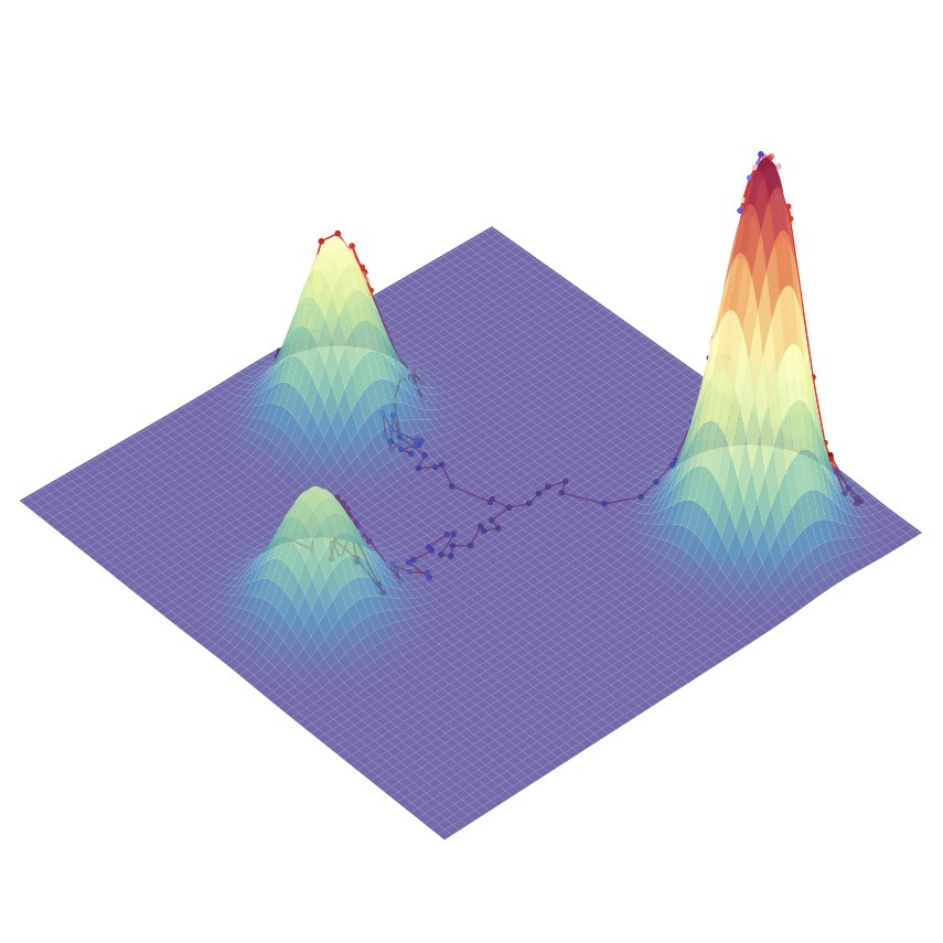
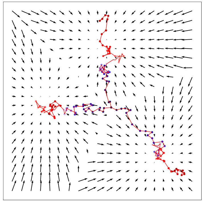
$x_0$는 real data의 분포에서 random하게 sampling한 값이고 $\epsilon \sim \mathcal{N}(\epsilon;0,I)$는 extra noise term으로 생성되는 sample들이 mode collapse되지 않도록 하면서 mode 주위를 맴돌도록 해주는 역할을 합니다. (즉 똑같은 이미지를 생성하지 않으면서도 mode(최빈값)에 가까울 수록 더 자연스러운 이미지일테니 이 주위를 맴도는 sample을 추출하도록 하는 역할입니다.) 또한 학습된 Score function은 Deterministic하기 때문에 생성 프로세스에 Stochastic한 값을 추가하여 이를 우회하는 의미도 있습니다. 예를 들면 아래 그림처럼 mode가 2개일 때 유용하게 작용할 수 있습니다.

3개의 Mode가 있을때 Stochastic 하게 sample을 추출하기 때문에 각 Mode에 해당하는 sample들을 모두 추출할 수 있습니다.

 

다만 여기서 ground truth score function은 우리가 예측하기 힘든 real data의 매우 복잡한 분포를 가지고 있습니다. 다행히도 우리는 score matching을 통해 ground truth score 없이도 Eq 157의 Fisher Divergence를 minimize 할 수 있습니다.